


Introduction
Clustering is used to identify and classify into groups of similar objects in a multivariate data sets. It locates the centroid of the group of data points in the dataset to classify.
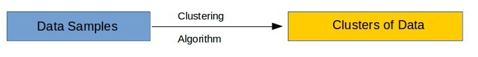
Fig 1.
When a data set of items, with certain features and value is to be categorized, we can use k-means algorithm. This unsupervised learning algorithm will categorize the items into k similar groups. To calculate that similarity, we will use the Euclidean distance as measurement.
Applications
k-means finds application in various fields such as marketing, medical, and computer vision. To name a few, detecting cancerous cells, color quantization to reduce the size of color palette of an image, image segmentation, and categorizing customers behavior. For better understanding color quantization application is described below.
Color Quantization Application
Color quantization is one of the primitive technique of lossy compression. Pixel-wise color quantization of an image shall be achieved by k-means. The pixels that are represented in the 3D space shall demand 3 bytes per pixel. Using k-means, the number of colors required to represent an image, shall be reduced. As a result, the file size is also reduced.
The Quantized image shown below is the result of k-means clustering with 64 centroids. This file size is reduced to 1/3 of original image size.
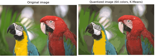
Fig 2.
Advantages
- Easy implementation with computationally fast and efficient with large number of variables
- Works well with distinct boundary data sets.
Disadvantages
- Difficulty in predicting the exact k-value for unknown data set.
- Initial seeds have a strong influence on the final resulting cluster.
Algorithm
- Initialize k points, called the ‘centroid’, randomly or from the data set.
- Data Assignment Step – Group all data points individually with its nearest centroid to form the clusters.
- Centroid Update Step – Calculate the value of centroid that is the average of items belonging to each cluster.
- Reiterate step 2 and 3, till the centroid value remains constant between consecutive iterations.
Flow Chart
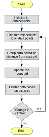
Fig. 3
Illustration
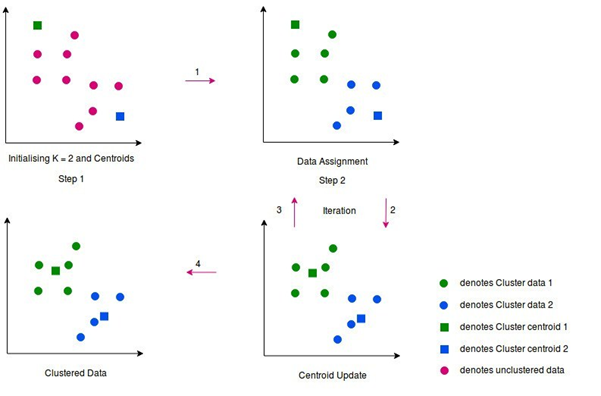
Fig-4
Experiment Sample Data
We are going to do an experiment now with sample random data set applying k-means clustering.
Each Iteration strives improving the accuracy as explained earlier, and finally we get the data clustered, and further iteration stops improving.
Data-Set: { 10, 11, 15, 15, 19, 20, 20, 21, 22, 29, 30, 40, 45, 46, 51, 60, 62, 62, 62}
lets assume the k value is set to two (k = 2), and cluster the data. As it is the intial iteration, we choose randomly the centroids 15 and 31. When applying the algorithm with these centroid value, new centroids are computed. The new Centroid values are 17, 48.7 as shown in Fig-5
Iteration 1
| Data Points | Centroid 1 | Centroid 2 | Distance from Centroid 1 | Distance from Centroid 2 | Nearest Cluster | New Centroid |
| 10 | 15 | 31 | 5 | 21 | 1 | |
| 11 | 15 | 31 | 4 | 20 | 1 | |
| 15 | 15 | 31 | 0 | 16 | 1 | |
| 15 | 15 | 31 | 0 | 16 | 1 | |
| 19 | 15 | 31 | 4 | 12 | 1 | 17 |
| 20 | 15 | 31 | 5 | 11 | 1 | |
| 20 | 15 | 31 | 5 | 11 | 1 | |
| 21 | 15 | 31 | 6 | 10 | 1 | |
| 22 | 15 | 31 | 7 | 9 | 1 | |
| 29 | 15 | 31 | 14 | 2 | 2 | |
| 30 | 15 | 31 | 15 | 1 | 2 | |
| 40 | 15 | 31 | 25 | 9 | 2 | |
| 45 | 15 | 31 | 30 | 14 | 2 | |
| 46 | 15 | 31 | 31 | 15 | 2 | 48.7 |
| 51 | 15 | 31 | 36 | 20 | 2 | |
| 60 | 15 | 31 | 45 | 29 | 2 | |
| 62 | 15 | 31 | 47 | 31 | 2 | |
| 62 | 15 | 31 | 47 | 31 | 2 | |
| 62 | 15 | 31 | 47 | 31 | 2 |
Fig-5
Now, we repeated the algorithm with previous iteration centroid values, and this results the new centroid values 19.27 and 53.3 as shown in Fig-6
Iteration 2
| Data Points | Centroid 1 | Centroid 2 | Distance from Centroid 1 | Distance from Centroid 2 | Nearest Cluster | New Centroid |
| 10 | 17 | 48.7 | 7 | 38.7 | 1 | |
| 11 | 17 | 48.7 | 6 | 37.7 | 1 | |
| 15 | 17 | 48.7 | 2 | 33.7 | 1 | |
| 15 | 17 | 48.7 | 2 | 33.7 | 1 | |
| 19 | 17 | 48.7 | 2 | 29.7 | 1 | |
| 20 | 17 | 48.7 | 3 | 28.7 | 1 | 19.27 |
| 20 | 17 | 48.7 | 3 | 28.7 | 1 | |
| 21 | 17 | 48.7 | 4 | 27.7 | 1 | |
| 22 | 17 | 48.7 | 5 | 26.7 | 1 | |
| 29 | 17 | 48.7 | 12 | 19.7 | 1 | |
| 30 | 17 | 48.7 | 13 | 18.7 | 1 | |
| 40 | 17 | 48.7 | 23 | 8.7 | 2 | |
| 45 | 17 | 48.7 | 28 | 3.7 | 2 | |
| 46 | 17 | 48.7 | 29 | 2.7 | 2 | |
| 51 | 17 | 48.7 | 34 | 2.3 | 2 | 53.5 |
| 60 | 17 | 48.7 | 43 | 11.3 | 2 | |
| 62 | 17 | 48.7 | 45 | 13.3 | 2 | |
| 62 | 17 | 48.7 | 45 | 13.3 | 2 | |
| 62 | 17 | 48.7 | 45 | 13.3 | 2 |
Fig-6
Having repeated once more with previous centroids, , we see the newly computed centroid values are again set to 19.27 and 53.3, as shown in Fig-7.
Iteration 3
| Data Points | Centroid 1 | Centroid 2 | Distance from Centroid 1 | Distance from Centroid 2 | Nearest Cluster | New Centroid |
| 10 | 19.27 | 53.5 | 9.27 | 43.5 | 1 | |
| 11 | 19.27 | 53.5 | 8.27 | 42.5 | 1 | |
| 15 | 19.27 | 53.5 | 4.27 | 38.5 | 1 | |
| 15 | 19.27 | 53.5 | 4.27 | 38.5 | 1 | |
| 19 | 19.27 | 53.5 | 0.27 | 34.5 | 1 | |
| 20 | 19.27 | 53.5 | 0.73 | 33.5 | 1 | 19.27 |
| 20 | 19.27 | 53.5 | 0.73 | 33.5 | 1 | |
| 21 | 19.27 | 53.5 | 1.73 | 32.5 | 1 | |
| 22 | 19.27 | 53.5 | 2.73 | 31.5 | 1 | |
| 29 | 19.27 | 53.5 | 9.73 | 24.5 | 1 | |
| 30 | 19.27 | 53.5 | 10.73 | 23.5 | 1 | |
| 40 | 19.27 | 53.5 | 20.73 | 13.5 | 2 | |
| 45 | 19.27 | 53.5 | 25.73 | 8.5 | 2 | |
| 46 | 19.27 | 53.5 | 26.73 | 7.5 | 2 | |
| 51 | 19.27 | 53.5 | 31.73 | 2.5 | 2 | 53.5 |
| 60 | 19.27 | 53.5 | 40.73 | 6.5 | 2 | |
| 62 | 19.27 | 53.5 | 42.73 | 8.5 | 2 | |
| 62 | 19.27 | 53.5 | 42.73 | 8.5 | 2 | |
| 62 | 19.27 | 53.5 | 42.73 | 8.5 | 2 |
Fig-7
Final Centroids = 19.27 and 53.5
Looking at the result of iterations, last two iterations continued to have same centroid values (19.27 and 53.5). This essentially indicates, there can’t be any more improvement, and hence these centroids are considered final values. By using k-means with k value set to 2, obviously 2 groups have been identified that are 10-30 and 40-62. It is worth mentioning that the initial choice of centroids shall affect the output of clusters, and hence the algorithm is often run multiple times with different initial values in order to get a fair clustering.
Best Fits
Works well with non-overlapping clustered data sets with a smaller number of outliers and noise.
k-means algorithm finds the local minimum solution and not the global optimal solution, that is, the solution is based on initial condition. The effect of variation of cluster can be minimized by running the algorithm multiple times by changing the initial seed. The cluster that gives minimum cost function that is Euclidean distance or variance can be taken as the optimal cluster.
Choosing K Value
In general, there is no method for determining the value of K, but an approximation k value shall be estimated by applying different k values and projecting the results into the graph as shown below. Variance as a function of K is plotted and the “elbow point,” where the rate of decrease sharply shifts, can be used to find K. The plot shows the transition from extremely low number of cluster centroids to a high number of centroids. The elbow in the diagraion Fig-8 signifies the optimal k-value (number of clusters).
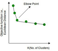
Fig-8
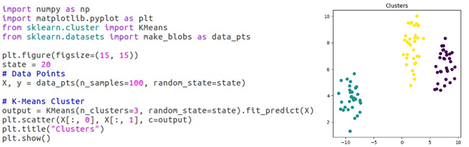
Clustering using Scikit
Reference
J.B. MacQueen (1967): “Some Methods for classification and Analysis of Multivariate Observations,
Proceedings of 5th Berkeley Symposium on Mathematical Statistics and Probability”, Berkeley,
University of California Press, 1:281-297